Machine Learning for the Markets

Traditional technical analysis is like interpreting constellations in the sky. Connect a series of dots (pivots) to find an interesting pattern such as a head-and-shoulders formation or a beautiful butterfly, and then supposedly the pattern is either bullish or bearish.

Many technicians spend their lives chasing the Holy Grail: a system that will make them rich simply by detecting common patterns and executing trades just by following a special recipe. Technicians in history such as Edwards, Elliott, Fibonacci, Gann, and Gartley showed us visually appealing charts but no evidence that these techniques actually worked.

Once you come to the conclusion that there is no master algorithm, then you can move to the next level. Collectively, technical analysis is really just an infinite set of features to use in training models. Further, we have discovered that all of the systems you need have already been invented. The real magic is then using machine learning to decide which system to deploy at any given moment.

Systems generally operate in two contexts: trend and counter-trend. You can run a system such as Toby Crabel’s Open Range Breakout (ORB) for Widest-Range (WR) days where you think the market or instrument is going to trend, or alternatively you can fade support and resistance in a mean-reverting strategy. [Note that Mr. Crabel runs a successful hedge fund and wrote a rare, groundbreaking book on short-term trading: Day Trading with Short Term Price Patterns and Opening Range Breakout]

Clearly, you will lose money by blindly executing any short-term system on any given timeframe. About twenty years ago, when artificial intelligence was first hot, some funds tried their hand but failed. The problem was that using neural networks to predict positive return was misguided. Instead, you need a bidirectional strategy that goes short as easily as it goes long, but in the proper context.

So, when we build our machine learning models, we have a wide range of dependent or target variables from which to choose, not just net return. There is more power in building a classifier rather than a more traditional regression model, so we want to define binary conditions such as whether or not today is going to be a trend day, rather than a numerical prediction of today’s return.

Back to our example, let’s look at a Crabel pattern WR4 on a daily basis (Widest Range with 4 indicating the rolling four-day period). We want to train a model that predicts whether or not any given day will have the widest range in the past four days. If our trained model gives us any kind of predictive power, then we can screen out the Narrowest Range (NR) days and avoid trading the ORB system by cutting out the losing trades. We want to locate WR4 patterns with fairly high accuracy.

First, a note about imbalanced classes. If the pattern you’re trying to predict is rare, and you’re trying to achieve the best accuracy, then training a model will be generally useless because the classifier will be biased towards predicting the majority class. I prefer to get as much data as possible and then under-sample the majority class so that the resulting classes (training labels) are equally balanced.

Training the data using Random Forests and XGBoost, we obtained the following results on our test sets:

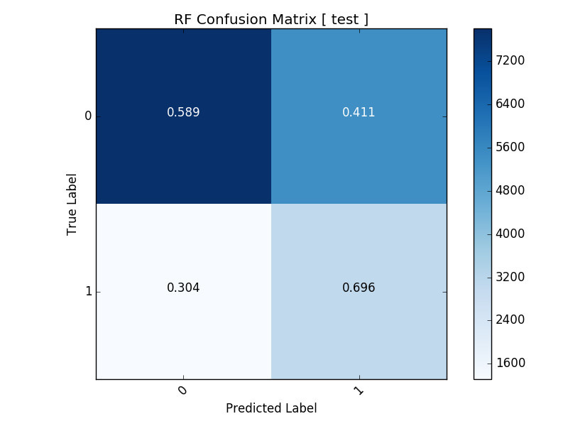
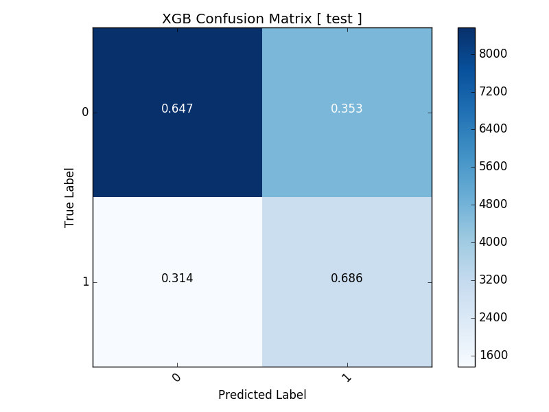
For either algorithm, we can predict WR4 days with almost 70% accuracy. Consequently, we can then define our own trading regimes to select which system is most appropriate at the beginning of every trading day. We can also experiment with these models at different fractals, such as weekly or even intraday on an HFT (High Frequency Trading) level.

Let’s now examine the feature importances to see if both algorithms are picking up commonly significant features:

Of the top 10 features, we have 5 shared important features, although not in the same order or magnitude: 17, 42, 109, 110, and 130. Still, these bar charts of the relative importance of each feature bolster our confidence in the model.

Before deploying any model in real-time, we want to assess the degradation in the model between the training and testing set. For classifiers, I prefer both the ROC (Receiver Operating Characteristic) and the calibration curves. First, here are the ROC curves:

You can see that the mean of the AUC (Area Under Curve) decreased from 0.87 in the training set to 0.71 in the testing set, as expected. Now let’s compare the confidence levels when we calibrate each classifier. We want to make sure that all of our calibration curves slope upward from left to right.

The perfectly calibrated classifier would yield a straight line, but we still see that even in the test case, the curves slope upward. So, which algorithm is best? The lower-right graph shows the distribution of the mean predicted value [deciles of 0.1] for RF and XGB. Clearly, the distribution of XGB counts (green line) is more uniform, so that gives us more confidence. In contrast, the RF decile counts are quite small at either tail. I prefer to use XGBoost in most cases, as its reputation is stellar, and it has won many Kaggle competitions.

For practitioners of technical analysis, all is not lost. The point of machine learning is to build useful models from data, and technical analysis is just that: data. But you no longer have to experiment with just a few variants of RSI or MACD on your charts. You can just dump thousands of these technical indicators into the feature blender and see what comes out.

As I was finishing this article, I saw a trader’s note that a stock was about to “break out of its saucer”, a visually alluring premise. Yes, technical analysis can be beautiful with its charts and formations. But in the long run, machine learning is going to crush it.